
CONTENTS
of Compass Points 22
The journal of the BCRA Cave Surveying Group.
Why don't you come to field meets?
SNIPPETS
John Lyles, Steve Taylor
*Thilo Müller
Report of the seminar, covering version 3.0 of CAD für Höhlen and also Toporobot.
Phil Underwood, Anthony Day
Two opinions of the Silva prismatic-lensed instruments.
*Wookey
Martin Sluka's addition of a laser pointer to a geologic compass
Andrew Atkinson
*Bernie Szukalski
Andy Atkinson describes the progress and process of the UIS symbols commission.
SOFTWARE UPDATES
Olly Betts
Olly describes some proposed changes to the Survex command line in the light of its evolution since 1991.
The new visualisation software is now available to the public.
Bernie Szukalski
A new release of the companion tools for Compass
LETTERS
*Stuart France
Stuart describes a nifty alternative to mounting lights on your instruments.
CSG Field Meet Reports:
Julian Todd
Julian describes how a sample cave was surveyed and entered into Tunnel to test it. Some problems with the implementation were revealed and subsequently fixed.
Wookey
How to improve your Suunto so that it can be more easily disassembled and maintained.
Dave Gibson
David Gibson describes a novel method of radiolocation that could give rise to a new tool for cave surveying.
I’m going to witter on about field meets a bit this issue. This last meet was very interesting, but it was very noticeable that almost everyone there was CUCC, or ex-CUCC. This makes for a pleasant weekend, but isn’t really what we were trying to achieve. So, why did you all stay away? This meet was set a long time in advance and well-trailered in CP, Caves & Caving, Descent, the BCRA/NCA diary and the BCRA conference, so people who might want to go presumably knew about it. So, maybe there aren’t any surveyors outside CUCC, they were all doing something else that weekend, or the program didn’t appeal.
We would really like to hear from people with any opinions about field meets. Why didn’t you feel like coming to this one? What would make you want to come? Was it the wrong venue? Do you want more details in advance of what might be going on? Do people want field meets at all? Is twice a year too often? Please give us some feedback. Otherwise we’ll just continue as we are, because we don’t know what else to do, and those who did turn up had a good time.
BCRA Conference - Hidden Earth
The CSG had a stand with display board and computer. Demonstrations of Tunnel were very popular, as were updates to version 0.80 of Survex. The display included the UIS cave symbols list, and information about the CSG’s archiving project. We were hoping for some feedback on both of these but I didn’t get any, except on the latter at the AGM.
Wookey won the Arthur Butcher survey award: ‘The award panel was impressed by Wookey's contribution ,to the development of surveying techniques and especially by his enthusiastic promotion of cave surveying ideas and knowledge through the Cave Surveying Group, which he helped to form and whose newsletter he edits. Wookey wins an annual trophy; plus Waterproof notebooks and pen from Weatherwriter and Swildons Survey from Wessex CC.
His response: I must admit to being quite pleased to get this. The actual miner’s dial is of course pretty useless, and just hangs around the mantlepiece until next year, but it’s really nice to have one’s efforts recognised, as editing CP can feel like a bit of a slog sometimes. The notebooks are good too J
Forthcoming Events
Spring CSG field Meet
The next field meet will be in the south, in one of Mendip, Forest of Dean or Wales. If anyone wants it to be in their hut, so they don’t have to go far to attend, then please contact Andy Atkinson, so we can make a booking. Also note the comments in the Editorial about field meets. Any and all opinions about what should go on are most welcome.
CSG AGM
We had our AGM at the BCRA conference. This was a typically informal affair mostly concerned with a very useful discussion of ways to progress the Survey Archive. Andy Atkinson has found that microfiching works very well, and is cost-effective and durable for archiving, and the basic rules under which information is kept are also largely agreed. That still leaves big questions about the actual physical & electronic storage of documents (ie how and where), the mechanisms by which people would gain access to information, and who would pay the costs. Several sensible things were suggested, including approaching Education Research Councils and the Millenium Commission for money, and seeing if other established organisations such as the Limestone Research Group or the BCRA library would be interested in providing storage space and filing. There were also useful ideas about putting some of the data on CD for distribution or publicly available information, and as a long-term storage medium, perhaps using CDR to send out information to particular groups.
All these suggestions will be followed up in due course.
First, a couple of items from the cave-surveying mailing list:
Cheaper Disto
A new flyer just came my way, from EPD Technologies, in Elmsford, New York. (800) 892-8926.
They are listing the Leica Disto Basic Laser Rangefinder for $895 US dollars now. Last spring it cost $1300 from local surveyor stores, as Carlsbad Caverns bought two of them, for use in measuring distance. The Disto Basic has an accuracy of +/- 0.2 inches, and range from 1 to 300 feet, depending on the target conditions for the laser spot. On natural surfaces expect reliable operation to about 100 feet.
At the present rate, these things might be affordable after the Christmas holidays here.... Well, affordable is all relative, still a lot more $$ than a tape to measure distance. Also, the old tape is a lot more indestructible for caving, even slimy, muddy caves.
Site for UTM/Lat-Long conversions
A site that my be useful if your locality is in UTM and you want to use one of the Lat/Long declination sites in the preceeding post.
http://internetgis.com/utm/utm.html
[This prompted an extremely pedantic discussion about whether, in fact, all localities were in UTM, and if so, how far off the surface of the earth this applied - some of us should get out more J ]
Cave surveying seminar in Hallstatt Obertraun 1998.11.6-8
Thilo Müller (translated by Mark ‘Doc’ Morgan & Wookey)
Some 30 participants from Austria, Germany and Switzerland spent the weekend in Obertraun, Austria, at the invitation of the Hallstatt Caving Club. The principle presentations were of the latest versions of ‘CAD for Caves’ by Tobias Bossert, and ‘Toporobot’ by Martin Heller. Additionally, there were lectures on the 3D-representation of caves, and discussions about other programmes such as Survex and Smaps.
The updated version of Toporobot was presented by Martin Heller from Zurich, but since this first class programme is already well known it will not be gone into in detail here. Some points, however, were not familiar to all participants of the seminar, and so will be expanded upon here. While Martin would prefer the strict notation of the internal station names to be maintained, it is possible for the user to use any station names if he wishes. This is particularly advantageous during the entry of older survey data. Furthermore, in the next weeks/months it is expected that a fully operational version of Toporobot will be available for the PC. As always, Martin impressed with new features during his 3D demonstration of cave surveys.
Tobias Bossert presented version 3.0 of CAD for Caves, which should be finalised in the coming spring. It will then be compatible as an application for AutoCAD 14 (on Win95), which will show substantial improvements in relation to the previous versions. Thus generally user-friendliness improved significantly and by giving up the support of older AutoCAD versions can it does everything that could be done with version 14. The application is written in German.
Interestingly, it is now possible to insert cave details such as rocks, mud & boulder chokes, semi-automatically. No longer does it have to be gone over again - the insertions adapt to the available border lines automatically, unlike earlier versions. By refined algorithms Tobias has succeeded in making the inserted details look almost hand drawn, and not at all regular.
A further improvement is the omission of the tablet, as the available draft plans can now be scanned and displayed as a bit-map in the background. These can then easily be digitised with the mouse from the background.
The extended layer system allows, in the future, the addition of as many caves as is desired to a drawing and yet to still address all individual layers separately or together e.g. all ‘mud’ layers of the respective caves together, or each different layer within a cave. This gives unlimited possibilities during the selection and representation of the individual items.
As a major task of the application, apart from the simplified insertion of pre-defined drawing blocks, Tobias sees the structuring of the data by the layers, on which the individual items are stored. From this also comes the main use of CAD systems, i.e. the output of cave plans for different purposes or effects e.g. to answer the following questions: Where I find sediments? Where do streams flow? Where are calcite deposits? Where are technical installations? Also output at different scales is supported, since text and symbol densities are adapted to the scale.
In the course seminar it turned out that without too much effort both programs can be co-ordinated by means of a data interface (structured dxf files). In addition Martin and Tobias want to agree in the coming time on the details. Afterwards Tobias will not continue to support its input program (Lotus 123), but instead expect a dxf input file from Toporobot. Thus a complete data path would, probably for the first time, be created, which allowed the creation of a completed survey with all the steps in the computer from the data acquisition, calculation, 3d-visualisation and printing.
CUCC borrowed a pair of these for this year’s expedition, and we also took them to the field meet to try out. Here are a pair of opinions on how they compare to the conventional Suunto lensed instruments. (thanks to Nick Williams for the loan)
I used the Suunto compass and clinometer whilst surveying part of Schwarzmooskogeleishöhle, (Loser Plateau, Totes Gebirge, Austria). These units are viewed with through a prism attached to the top of the dial, rather than the usual window in the end most of us are used to. I found them easy to light with a pen-torch (they had no built-in illumination).
I actually found them very easy to use - the numbers were nice and large. They did not seem to mist up like lens-adapted instruments, which is always a problem, especially I feel in Austria.
There are, however, some disadvantages. The prisms stick out from the body of the instruments, and I did worry a little about knocking vital bits off. Also, these prisms look as if they could be painful if they were kept next to your body in tight squeezes.
All in all, however, I liked these instruments. Good gear!
I'd better write down my impressions gained of the compass/clino set I was using at the weekend.
One general thing is that they were only graduated in whole degrees, not half degrees. That apart, the compass was great - very easy to read, though difficult to judge when it was level (probably because I'm used to using lensed Suuntos), and I would prefer a cross hair rather than the pointer from above that it had. Even so the pointer was very clear (didn't seem to mist up either, despite all the water that was floating around.)
As for the clino, I had difficulty spotting the cross hair [in fact the cross hair had disappeared on this instrument - it is normally very clear - Ed]; the scale was smaller and hence harder to read than the compass. There were two main problems. First, because the sight is on one side, I found I had to sight on the point with my left eye and read the scale with the right all the time - if sighting with the other eye, the body of the clino got in the way (with practice it may well be possible to resolve this.) The other problem was lighting the thing - it seemed like I had to get the lighting angle just right otherwise the scale was invisible (also had to be lighted from the same side as my head was - leads to a bit of a space problem when the station is on the LH wall).
WeatherWriter waterproof notebook review
Wookey
Weatherwriter, suppliers of equipment and stationary for outdoor use, sponsored the BCRA conference with waterprrof notebooks, memopads, tyvek laser-printer waterproof paper, and pressurised pens.
The CSG tried out the waterproof notebook on the field meet, surveying Dowel Dale Side Pot. There were two teams, one using the ‘WaterBook’, the other using a Chartwell Rag-paper notebook. The bottom half of Dowel Dale was ‘pretty damn wet’ for surevying on that day. Water dribbles out of all the holes in the choke so it’s almost impossible to keep the notebook dry after a while. The normally excellent rag-paper really wasn’t up to the job, as all the pages became stuck together and it slowed surveying down significantly. It didn’t disintegrate or lose the data, but it wasn’t much fun.
In contrast the Waterbook was excellent. It retained pencil in the wet and dry very well, and the sopping conditions had no effect whatsoever on its use. The surveyors were instant converts. Washing the mud off afterwards was easy and left the data very clear. There was none of the problem that some waterproof papers have where the pencil comes off nearly as easily as the mud & water. The physical format is a plastic backboard with a wire-binding. The similar Waterbook Memopads are made of the same paper, but would need some kind of support for cave surveying as the books are floppy on their own.
Survey compass with laser pointer.
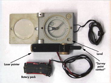
Martin Sluka's compass with attached laser pointer
Martin Sluka, from the Czeck Republic, has improved his surveying compass by adding a laser pointer. This is mounted on the side on a brass bush so that it can rotate vertically. This allows the compass to be levelled but the laser pointer to show the direction of the shot, making steep legs much more accurate. The added parts are all non-magnetic, containing only the laser diode taken from a normal lecture-room laser pointer. The batteries are on a wire so that they are kept away from the compass.
After lots of tedious debate, we are at the final stage of voting for the international symbols list.
The idea is that these will form the basic set and then individual drawers may add their own if they find it necessary. These should then be included in the key.
The main changes from the original list are:
Plan: 
Elevation:


All those changes are available on the Webpage at
http://www.gis.univie.ac.at/strv/strv/leute/andi/caving/cave-symbols/english.html
The voting works like this:
Each country has one voice. Countries that don't vote explicitly are assumed to vote for the present list. The simple majority (51% of all countries) wins, if there's equality the president decides.
The list of official delegates is as follows:
France Jean-Pierre Aulas
Oesterreich Andreas Neumann
Schweiz Philipp Haeuselmann
Deutschland Ralph Mueller
Russia Igor Lavrov
Brasilien Rubens Hardt
Australien Ken Grimes
UK Andy Atkinson
USA Garry Petrie
Argentina Redonte Gabriel
Venezuela Alvaro Rangel
I am the only one that may vote for the UK, let me have your comments.
Just so people know were I stand, and the default position if no one contacts me, I feel that generally the symbols are acceptable but there are too many things to balance, mainly national individualism, with lack of compromise. I will abstain but try to use the symbols in the future.
[The vote was taken in September (this piece was written before then), so it’s too late to change things now (Hidden Earth was your last chance). Ed]
Survex version 0.80 released
Olly Betts
Survex’s home on the Web has moved to its own domain at http://www.survex.com/ which should be easy for you all to remember, and Wookey and Olly can be emailed as olly@survex.com and wookey@survex.com.
Many changes - here are the most notable:
Various other things are in the works at the moment. These include blunder detection, and a native NT version of Survex (both of these are already working in ‘experimental’ form). Also mooted is a win32 version of caverot so it can run natively using DirectX. We also have some fairly rough converters using Perl for SEF -> Survex and Survex <-> CDI (for Comapss and Onstation). These should make it much easier to transfer data between applications, and will go up on the website when they are a bit more ready.
The following piece is derived from recent discussions on the Survex Mailing list, however I think it is worth repeating here for those who use Survex, and thus may be affected by the changes, but are not on that list.
Proposed Changes to Survex
Olly Betts
I've been updating and rearranging the documentation (I'm still working on it, but a recent snapshot is available at http://www.survex.com/docs/).
While working on this, it's become increasingly clear to me that the command line options to survex are in real need of an overhaul. Hopefully this can be achieved with minimal disruption - what follows is a brief summary of the problems with the current situation, followed by a sketch of what I have in mind. Finally I'll indicate how you might have to adapt existing datasets.
There's something of a balance to be made between fixing aspects of Survex which in retrospect aren't so good, and breaking compatibility with existing users. I'm hoping I can tidy up this (and any other problems) before we get to version 1.0 without annoying anyone, so please speak up if you have any opinions on these changes. Likewise, let me know if there are any aspects you think need attention.
Problems
The need to sometimes use both ".svx" and ".svc" files just complicates matters unnecessaryily.
The "@" alias to "-f" doesn't work as intended on the standard DOS version (since the DJGPP C runtime handles @ itself in a slightly different way).
The use of "!" to negate boolean options is very unhelpful under UNIX as many UNIX shells interpret "!" as an instruction to recall (parts of) previous commands. So the user has to enter: survex -\!p slimepit
The use of "(" and ")" on the command line is similarly problematic for UNIX users.
Except on UNIX, command line options may be started with "/" (as well as the UNIX style "-") which just seems to hinder providing a uniform interface to users. The intention was to be consistent with DOS tools using "/", but I don't think that's important (other DOS tools aren't consistent anyway).
Supporting both "-" and "/" on all platforms isn't a solution, since a full UNIX path begins with "/".
The case insensitivity of command-line options halves the number of potential one letter options (this is partly a DOS vs. UNIX philosophy clash really).
The -U (uniqueness) option is now misnamed as it actually controls truncation (as of version 0.80).
Options like "-C" (case insensitivity), "-N" (ninety to up), "-U" (truncation), and "-T" (title) are really part of survey data. "-A" (ASCII 3d file) and "-P" (display percentage complete) control the run and the output format. It would be clearer if some distinction was made between these two different groups of options (though this could be addressed in the documentation).
It would be nice to offer "long form" options as an alternative to the cryptic single letter options (like many modern UNIX tools do).
Suggested solution
Reduce survex command line options to:
-a --ascii-3d-file (deprecated[*])
-d --data-file (needed to process a survex filename starting with a "-")
-p --no-percentage
[*] The replacement for the .3d format won't provide ASCII and binary variants, so the "-a" option won't last for long. In case anyone needs ASCII .3d files I'll keep the option for now.
There's no real need to be able to negate any of these options, but for any future options which do need to be negatable --frobnicate would negate to --no-frobnicate.
"@" goes (since "-f" does). So do "(" and ")".
The command line options used to do stuff in .svc files are turned into *-directives which can be used in .svx files:
*case (preserve|tolower|toupper) (was -!C/-CL/-CU)
*truncate (<n>|off) (was -U<n>/-!U)
*title <title> (was -T <title>)
*inferplumbs (on|off) (was -N/-!N)
(I may not implement these quite as described, but this conveys the idea).
If multiple files are specified on the command, settings changes will be contained within each (i.e. as if all .svx filenames were in "(" and ")" with the current scheme).
Where appropriate, these changes would be applied to caverot and the other programs, but the impact there is much less.
Changing existing data sets
Many users won't have to change anything (except maybe to use "-p" instead of "-!p" or "-!P" to suppress percentages when sending output to a file).
Something like: survex ( caveone ) ( cavetwo )
Becomes: survex caveone cavetwo
In general, a complicated command line (or .svc file) will become a small .svx file. So the example from the documentation:
survex Defaults ( SomeCave ) ( NewBit )
would become:
*include Defaults
*begin
*include SomeCave
*end
*begin
*include NewBit
*end
It might be best to rename survex to something else (suggestions welcome!) and provide a wrapper called survex which supported the old syntax and called the new version with the appropriate options (maybe generating a temporary .svx file). This would also fix a potential source of confusion in the documentation between the Survex package and the survex program (i.e. survex.exe on DOS) itself.
Please let me have your comments on all this.
Tunnel Released
Tunnel, the Survex-compatible cave-visualisation tool, is now available. It has been featured in CP before, in preliminary form, and some of you saw it at the BCRA conference. It has now been significantly revised in the light of the trials at the field meet, and some instructions have been written, so it is ready for public release.
You can find it via the Survex web pages, or at it’s home:
http://www.goatchurch.demon.co.uk/tnmain.html
The download is only 140K, but you do also need a Java Runtime Environment, or Development Kit, which is 3.5 or 9Mb respectively. The Java you may have built-in to your browser is not sufficient, as it doesn’t allow things to write to your local hard disk.
CaveTools Version 2.0 for ArcView GIS Now Available!
The latest version of the CaveTools COMPASS Converter for ArcView GIS is now available free from:
http://www.mindspring.com/~bszukalski/cavetools/cavetools.html
CaveTools provides an easy way to convert COMPASS cave survey data for use with your GIS database and GIS software. CaveTools is an ArcView GIS extension which converts COMPASS plot files to ESRI shapefiles, and includes additional tools to register cave survey data to real world coordinates (e.g., GPS locations). CaveTools Version 2.0 requires ArcView GIS Version 3.0 or later (Win95/NT only), and creates standard (2D) shapefiles for use with ArcView 2.0 or later, ArcExplorer 1.0 or later, or other GIS software.
Version 2.0 includes support for COMPASS Sections, and other improvements and enhancements.
Coming soon: CaveTools Version 3.0 for ArcView 3.1 with direct import to 3D shapefiles for use with ArcView's 3D Analyst.
For more information on COMPASS visit:
http://members.iex.net/~lfish/compass.html
Press Roundup
The only thing I have had this quarter is an exhaustive list of survey symbols and details of surveying technique from Romania. Unfortunately my Romanian isn’t too hot (although it seems to be a fairly standard latin language), so it may be a while before I can usefully summarise it.
Re: Instrument Lighting
Stuart France
(mailto:Linetop@aol.com)
Dear Editor,
Further to your recent article in Compass Points, readers may be interested to know of a different approach which does not involve sticking things to instruments. What I've done is to provide an additional non-magnetic mobile light source on the helmet which can move into the exact position you need.
My power solution is to drive an ordinary LED (highly magnetic) with the Petzl-style helmet-mounted battery pack that I normally use for UK caving - but equally well it could be a small battery, say 2xAAA cells, stuck somewhere to the rear or side of the helmet.
The light from this remote LED is piped to the front of the helmet with a piece of fibre optic cable, leaving a dangly bit (15cm) coming through the brim of the helmet which can be poked equally well at the capsule of a compass or clino. I suppose you could modify your lamp headset so that some of its light is diverted through a piece of fibre optic cable.
More recently I've replaced the fibre optic with ordinary twin core copper cable and soldered a surface-mount LED (which is not magnetic at all) on the end of it and enclosed that end bit in epoxy. This works very well and you soon get used to the idea of holding the compass or clino and the dangling light beam at the same time.
I would try and send you some pictures, but things are very busy.
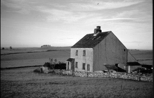
Abstract: The CSG held a field meet in Derbyshire on the weekend of 18th October. They went surveying and put the data into Tunnel to test its functionality in interfaces. They also learnt how to improve the fettleability of Suunto instruments, and saw the results of archiving documents on microtape.
Tunnel’s first cave
Julian Todd
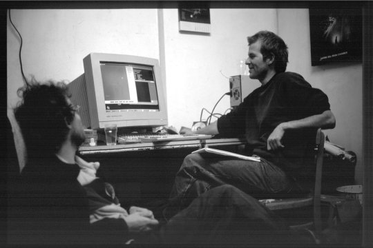
The Cave Surveying Group field meet in October was held at the Orpheus hut in Derbyshire. Eight people attended, all directly related to CUCC. Between us we brought three computers, two monitors and one mains cable.
One computer had no mouse, and of the other two, only a fairly ropey expedition computer running Wincrap 95 could be persuaded to execute Java and thence be able to run "Tunnel", the all-new cave tunnel modelling survey software that's compatible with "Survex".
The task for the weekend was to go and survey a cave, read it into Tunnel and see if we could construct some interesting results which could rival the claims we have made for the software in the past. When you go cave surveying, the data you collect depends on what you are going to do with that data. To construct a model of a cave passage, Tunnel requires precise cross sections to be mapped at key points in the cave, and then little tubes are connected between the cross sections to generate the image.
The cave to survey, Dowel Dale Side Pot, was chosen by Duncan (another CUCC person) who was not present due to wisely clearing off to Wales for the weekend. Dowel Dale is the Wednesday night futile dig for the local TSG cavers, mostly scaffolded, short, muddy and dangerous. Just in front of the entrance panel of wood (to keep the sheep out) there was a bright brown human turd pile dissolving into the ground. Evidently some passing walker had thought it was a secluded hollow nobody would be wanting to pass their time in.
We cleaned it up and spread gravel over it and then went in the cave. There were five of us. Becka and Anthony went to the bottom and surveyed out, while Wookey, Andy A and Julian surveyed inwards. The cave got progressively worse as we went in. Fortunately we had our little arguments about the theories of cross sectioning the passage in the slightly drier areas before we got to the really wet and dribbly bits where we would have been less inclined to have an intellectual debate. The party of two surveyed the cave in 16 legs and the party of three did it in 15 legs, and the cave was about 35m long.
Back at the hut we festered, lit the fire, powered up the computers and began to nerd. In the process we found several annoying features in Tunnel. The main one had to do with the way the cross sections were connected. Each cross section had four cardinal points on the profile, and these four points were supposed to connect to the corresponding four points on the next cross section. The points were roughly meant to be the Left, Right, Up, Down extremes, or even the West, East, North, South points on a horizontal cross section. Dowel Dale Side Pot had many vertical and horizontal parts to it, and switching between these different orientations caused the connections between the cross sections to have unwanted twists.
The other drawback with Tunnel is that only one cross section was allowed per survey station, and the plane of the cross section had to pass through that survey station. This didn't seem to be enough and the proposed solution of typing in fake survey stations on which to support intermediate cross sections was a pain in the neck. Intermediate cross sections along the tube connecting two survey stations were going to be necessary to avoid the prismatic look of the current output. The case we wanted to model was that of a passage snaking from side to side, but maintaining the same cross section.
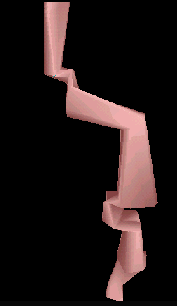
Figure 1 - Detail of Dowel Dale Side Pot, looking somewhat from above, with the scaffolded shaft on the right hand side.
 During the following week (since my boss was away) I fixed these two problems (and a few others) in the Tunnel specification so that what we have now is much simpler to comprehend and is complete. As far as what we imagined it could do, there are no missing core features. The only remaining things to add (like colouring parts of the cross sections, gluing features into the tubes, trimming back the tubes at junctions) are simply frills which will not be introduced until caves a bit more challenging than Dowel Dale have been tried out on the system to see how it currently performs.
Suunto refurbishment
We gathered in a wet and windy Derbyshire at the Orpheus hut. After the Saturday with actual caving in it we went for a slightly more relaxing Sunday, by driving off to Nick William's house in Great Hucklow, where he showed us how to make a suunto compass more easily serviceable. This is done by changing the eyepiece lens retention hardware.
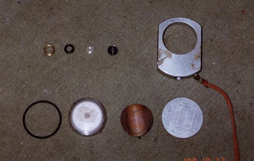
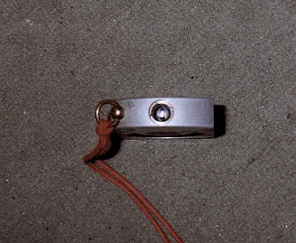
Normally the lens is held in by a friction-fit aluminium ring. This is very waterproof, but makes it almost impossible to get to the back of the lens to clean it, or remove condensation, because even if you take the back off and capsule out, the slotted shield behind the lens prevents access. Replacing the retaining ring with a removable threaded bush (Figure 1) makes it simple to disassemble the device completely for cleaning. Another advantage of having the instrument like this is that the lens focus can be adjusted by changing how far in the lens sits to deal with those annoyingly out-of-focus instruments.
In the bottom of the eyepiece hole there is a slotted brass piece (painted black) when gives the vertical slot that you look through to concentrate the attention an the area adjacent to the sighting hairline. Next is the lens (12mm diameter, 20mm focal length), and then the retaining ring. We keep the brass sighting slot and the lens, but then add a rubber O-ring followed by the threaded brass bush (Figure 2).
The procedure for this is simple but requires more equipment than most of us have to hand.
First you should take the back off and remove the capsule. The back is a friction fit that can be prised off (older instruments have a little slot to get your screwdriver into - on newer ones you can either make your own hole, or, if you don't mind possibly breaking the capsule, just push it out from the top. You remove this bit partly for access to the back of the sighting slot, and also to protect the delicate capsule from the violence the body is about to experience.
Then you have to extract the original retaining ring. You need a 7/16 UNF tap with the end ground flat (i.e. no lead-in threads). This is exactly the right size to screw into the retaining ring. The lead-in threads have to be removed because there is only about 4mm clearance above the lens. Screw the tap in until it has a good grip, but hasn't touched the lens. Now comes the fun bit! Hold the tap securely in a vice and then strike the instrument with a soft-faced hammer so as to pull the retaining ring out. You need to hit it quite hard, and this bit tends to chip the lens (presumably because the ring twists a bit before coming out. If you had a suitable puller to make sure the ring came out square, that might well preserve the lens better.
We are currently looking for a source for spare lenses, as if these were available at reasonable cost it wouldn't matter if you broke it. The only quote I have had so far was £25 for a too-big (15mm) lens plus £15 for grinding it down plus VAT, which is not very attractive!
Having removed the retaining ring you can take out the lens, taking care not to damage it any further. Then the sighting slot can be pushed out using a short rod to push it out from the capsule side. This shouldn't need much violence but is a bit stiff.
Now you need to put a thread in the instrument body to hold the new bush. This should be ¼"BSP, although no doubt a suitable metric size could be found. Tap down the hole, stopping when the tap reaches the shoulder that the sighting slot sits on, This leaves the bottom few millimetres more-or-less unthreaded so that the slot & lens still centre properly. Take a suitable diameter piece of brass tube. It needs to finish up being 13mm outside diameter, about 9mm inside diameter, and about 5mm long. Cut a ¼" BSP thread on the outside of the tube, drill the inside of the tube out to 9mm, cut it to 5mm length and then put a hacksaw cut across the centre of one end about 2mm deep, to allow a suitably sized screwdriver to be used to screw it in and out. The rear surface should be free of burrs as it will rotate on an O-ring when assembled.
Finally you can re-assemble the instrument. Put the sighting slot back in first (cupped end outwards), then the lens, then a 12mm O-ring, and finally screw the new bush in to clamp it down.
If anyone has any refinements to his technique or similar suggestions for improvements to instruments, the CSG would like to hear from you. If there is sufficient interest in this, it may be possible to arrange to get your instruments upgraded in this way for a small fee. Talk to Nick Williams or Wookey if you want to get this done and don't have the skills or equipment yourself.
After that little demo we retired to the nearby pub for beer, dinner and a CSG committee meeting.
Radiolocation using
Field Gradient Techniques
David Gibson
describes a novel method of radiolocation that could give rise to a new tool for cave surveying. He has won a nomination to present a paper on this subject at a meeting of the International Union of Radio Science at the Royal Irish Academy in Dublin, in December this year.Radio-location of cave passages using an induction loop is a standard procedure Essentially, a horizontal transmitter loop (vertical magnetic dipole) is placed underground and its location and depth below the surface are calculated by taking measurements using a receiver loop on the surface. A summary of the technique presently used by cavers is given below. The methods summarised here were described in (Gibson, 1996f).
1. Location of ‘Ground Zero’ (g.z.)
a) Location of g.z. by measuring the bearing of the field lines (i.e. the direction of the horizontal component) at several widely spaced locations.
b) Confirmation of g.z. by the absence of any horizontal field component.
Knowing g.z. the depth calculation for the subsurface transmitter is by one of…
Depth by absolute signal strength (AS)
This is, perhaps, the obvious method to use, but it depends on an accurate knowledge of the transmitter power. If the magnetic moment of the transmitter is
M and the received field strength is H0 then the depth, d is easily found from the inverse cube law of field strength v. distance to be ![]() (1)
(1)
Depth by field gradient (FG)
Confusingly, this is the method I referred to as ‘depth by signal strength’ in (Gibson, 1996f). With proper use of ratiometric techniques, an alternative ‘signal strength’ method can be made to work that does not require the transmitter power to be known. The field strength (say H0) at g.z. is measured and compared with the signal (H1) a short distance (y) above this. Using the ratio of these readings provides a convenient way of calculating the depth without needing to know the transmitter power or absolute gain of the receiver. The depth is given by
![]() (2)
(2)
This method is used in some commercial radiolocation equipment.
Depth by field angle (FA)
Most amateur designs by cavers have used measurements of the angle of the field lines as a method of depth determination. Away from Ground Zero the magnetic field lines are not vertical. By measuring the angle of the field to the ground (_a ), and knowing the distance to the ground-zero point (x), the depth of the transmitter can be calculated as
![]() (3)
(3)
This standard derivation was explained in (Gibson, 1998). A convenient use of the method is to find the distance x at which the field lines lie at 45_° to the ground. The formula then indicates that x/d _» 0.56, so the depth is approximately twice the distance x. Another technique would be to find the distance x at which the field lines were at 18.4_° , for which x/d = 1.
Enhancements to ‘Ground Zero’ Location Technique
As mentioned above, the standard method involves measuring field angle. This is tedious and requires a certain amount of skill. The antenna must be aligned with its axis pointing to g.z. and then tilted to obtain a null, and the angle measured.
One way to make this process easier would be to measure the field components using three orthogonal antennas together, and applying an algorithm. The technique for finding the field direction and angle of dip is similar to that described in (Gibson, 1996e). All that is required is for the antenna structure to be accurately levelled – it does not need to be aligned with Ground Zero.
As well as making it easier to obtain a reading, the use of stationary antennas to measure field component allows us to utilise a much lower bandwidth and so increase the distance at which we can operate.
It is not easy to use a very low bandwidth with a conventional nulling technique. The reason for this is obvious – if the bandwidth is B = 0.005Hz it is as if the signal from the antenna passes through a filter with a time constant of 32s (i.e. ½_p B) so when the antenna is moved it will take 32s for the signal level to substantially ‘catch up’. It is far easier to wait for two minutes for the signals to settle than try to adjust the position of the antenna to obtain a null in the presence of a 30s ‘lag’ to the signal. (Other things being equal, a reduction in noise-equivalent bandwidth from, say, 4Hz to 0.005Hz (800 times) would increase the signal/noise ratio by 29dB and the range by three times (i.e. 6_Ö 800).
In fact, not only is a narrow bandwidth useful, it is essential – the reason is that it allows the antenna to be made smaller. The traditional France / Mackin beacon as described, for example, by Mike Bedford (1993) would be a cumbersome, if not impossible, device to use in 3D. Brian Pease’s radiolocation antenna (Pease, 1996a,b), is lighter – and it demonstrates the advantage of a lower bandwidth. Utilising a digital phase-locked loop (Gibson – unpublished notes) would allow ferrite rods to be use in an even smaller, portable structure.
Even with a 3D stationary antenna, the field angle method still requires the operator to measure the distance to Ground Zero. However, we might suppose that measuring the field angle at three widely spaced locations (even without knowing the bearing of the field lines) should be enough to allow us to calculate the position of g.z. This is, in fact so, but measuring the field line angle is cumbersome, requiring a 3D antenna configuration. There is a simpler method.
We only need to use two co-axial antennas (e.g. small ferrite rods on a pole) to make a measurement of the vertical field gradient (as utilised in the FG method described in equation 2). If we were at g.z. we would use this measurement to determine the depth. If we were not at g.z. we could deduce that the underground transmitter must lie on a curved locus. Taking a number of readings would allow us to calculate the intersection of the loci and so determine g.z. and depth. This is similar to calculating the intersection of three bearings, but the algebra is not so straightforward.
Field Gradient technique
Using a standard notation, the vertical field strength at co-ordinates (r, _q ) from a horizontal underground loop transmitter is
![]() (4)
(4)
and we can derive the vertical field gradient (or to be precise, the gradient of the vertical component of the field) to be
![]() (5)
(5)
Although it is not immediately obvious, this expression is identical to equation 2 when _q =0 and y<<r.
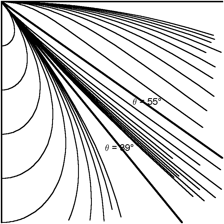
By making measurements of Hv and its gradient, we can say that the transmitter must lie on a locus of points (r, _q ) that satisfy the equation. Examples of possible loci are shown in the diagram above (from Gibson, unpublished notes), and it is the intersection of these loci, as measured at different receivers that allows us to fix the transmitter position. Two asymptotes are shown on the diagram; and there are other salient points, which it is beyond the scope of this short article to explain.
Thus, if we position three field-gradient receivers at surveyed locations on the surface then the data they collect will enable us to calculate the Ground Zero position of the underground transmitter and also its depth. This can all be done in one single operation.
Clearly the converse is also true – that with three surface transmitters (perhaps using orthogonal spread-spectrum codes) and an underground field-gradient receiver, the underground receiver can determine its co-ordinates – in three dimensions – at a single push of a button (and a short wait).
Construction of an adequate field gradient device requires a fairly high level of understanding of electronics but it is certainly possible. Some commercial radiolocation equipment already uses the FG method (but only for g.z. depth – not position); and Brian Pease has experimented with FG techniques and proved the concept.
Accuracy of Field Gradient Measurements
As already indicated, FG measurements do not require the skill that field angle measurements require. The field gradient is, however, affected by far-field distortion (Gibson, 1996f). The field line angle is also affected, and there is a more subtle effect, because the horizontal and vertical components become out of phase and it becomes more difficult to determine the null. The FG method could, if required, measure phase information as well as amplitude, and this information may be useful. But fundamentally, any accurate measurement using magnetic induction needs to be done at a distance of much less than a skin-depth. (And so, other things being equal, a beacon operating at 874Hz will give accurate results at 30 times the range of a radio at 87kHz).
Following my suggestion that the FG method be investigated, Brian Pease tried some locations at around 200m depth (Pease, 1997). Pease found that the FG method produced a smaller depth than the AS method. Checking this using a computer model (Shope, 1991) he made the interesting discovery that the FG method consistently underestimated the depth, whereas the AS method consistently overestimated; and that the mean depth given by these two results was remarkably close to the true depth.
For example, at 1000Hz and _s =0.01S/m the skin depth is 159m. Using Stephen Shope’s simulation package, for a depth of 320m, we find that FG would give a depth of 260m, whereas AS would give 392m – both significantly in error. However, the mean depth would be 326m – less than 2% in error.
Further analysis is needed here. Shope’s program suffers from iteration errors in certain conditions, so it would be unwise to use it to try to prove a point. However, it seems likely that a combination of FG and AS measurements (perhaps with phase and horizontal field gradient too) would allow us to get a reasonably accurate measurement under a wide range of conditions.
Anisotropic conductivity, mineralisation and other effects known to interfere with radiolocation will have an affect whichever method we choose to use. However, the nature of the FG method is such that we could choose to use a lower frequency and smaller bandwidth to try to reduce them.
The entire positioning system would appear to rely on accurately levelled antennas. An analysis of a tilted antenna in a FA system was given in (Gibson, 1998). Work by N.H. Nessler at Innsbruck University, Austria suggests that algorithms can be derived to deal with an unknown antenna tilt. So far he has not applied these to the field-gradient technique, but to other aspects of the problem of locating an underground transmitter in an unknown orientation (e.g. a body-mounted antenna on a trapped miner). I will report on this in the future.
I have described, in effect, a GPS device for underground location. As reported previously (Gibson, 1992) a ‘conventional’ GPS will not work underground because, even with local low-frequency transmitters to penetrate the ground, the time-of-flight of the signals is subject to wide variations dependent on the rock characteristics.
Measurement of field gradient using fixed antennas allows more accurate field measurements to be made, with a greater ease than the present field angle method.
A narrow bandwidth receiver allows a smaller antenna to be used and a greater range to be achieved. Readings will take several minutes to take but since the overall process is simpler and quicker this should not be a problem. Taking readings from three (or more) surface receivers, or using multiple surface transmitters and an underground receiver, allows a type of ‘global positioning system’ to be implemented.
Error caused by far-field effects will be addressed by analysis, but the problem is presumably no worse than for a field angle system.
Bedford, Mike (1993), An Introduction to Radio-Location, CREGJ 14, Dec. 1993, pp16-18, 14
Gibson – see list below
Pease, Brian (1996a) 3496Hz Beacon Transmitter & Loop, CREGJ 23, pp22-24.
Pease, Brian (1996b) The D-Q Beacon Receiver – Overview, CREGJ 24, pp4-6.
Pease, Brian (1997), Determining Depth by Radiolocation: An Extreme Case, CREGJ 27, pp22-25, March 97
Shope, Steven M. (1991) A Theoretical Model of Radio-Location, The NSS Bulletin, Vol. 53, No. 2, p. 83-88, Dec. 1991.
Further Reading
Articles on radio-location and surveying
by David Gibson)
All these articles will be placed on-line in the not-too-distant future – follow the radio-location link at
www.caves.org.ukGibson, David (1992), Global Positioning Underground, Cave Radio & Electronics Group Jnl. 9, pp18-20, Sept. 1992, ISSN 1361 4800
Gibson, David (1996a), Electronics in Cave Surveying, Cave Radio & Electronics Group Jnl. 23, pp25-26, March 1996, ISSN 1361 4800
Gibson, David (1996b), Review: Electronic Compass Modules, Cave Radio & Electronics Group Jnl. 23, pp27-28, March 1996, ISSN 1361 4800
Gibson, David (1996c) Electronics in Surveying, part 2, Cave Radio & Electronics Group Jnl. 24, June 1996, ISSN 1361 4800
Gibson, David (1996d), The Copyright of Cave Surveys, Caves & Caving 73, pp32-33, Autumn 1996 (Note 1), ISSN 0142 1832
Gibson, David (1996e), 3-D Vector Processing of Magnetometer and Inclinometer Data, Cave & Karst Science, 23(2), pp71-76 Oct. 1996 (Note 2), ISSN 1356-191X
Gibson, David (1996f), How Accurate is Radio-location?, Cave & Karst Science, 23(2), pp77-80, Oct. 1996 (Note 3), ISSN 1356-191X
Gibson, David (1998), Radiolocation Errors Arising from a Tilted Loop, Compass Points 20, pp11-12, June 1998, ISSN 1361 8962
Note 1: An earlier version appeared in Compass Points 11, pp5-7, March 1996
Note 2: This paper was given at the 1996 BCRA Science Symposium and a version appeared in CREGJ 25, pp18-22, Sept. 1996
Note 3: An earlier version appeared in Compass Points 10, pp5-9, Dec. 1995
![]()